First Order Motion Model for Image Animation (FOMM) を読む
First Order Motion Model for Image Animation
[A. Siarohin et al. NeurIPS 2019] という論文を読んでいきます (本文中の図は論文より引用)。
FOMMという名前で知られている手法です。
Method#
目的#
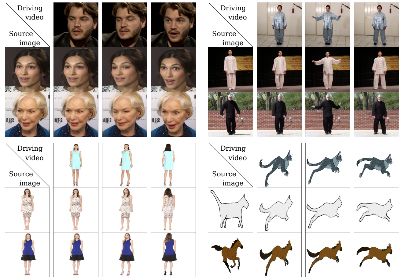
source image $\mathbf{S}$ と deiving video $\mathcal{D}$ の動きを表す潜在表現を組み合わせて、 driving video を再構成する
このとき、driving videoを同じような物体が写っている映像とすることで、教師なし訓練ができる。
概観#
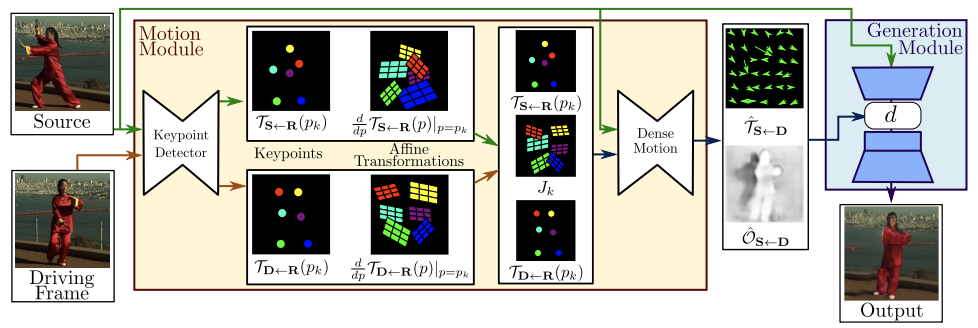
上図に本手法のoverviewを示す。inputは source image $\mathbf{S}$ と deiving video のフレーム $\mathbf{D}$ である。 それぞれに対し Keypoint Detector が 疎なキーポイント (sparse keypoints) と 局所的なアフィン変換 (local affine transformation) を抽出する。 そして、dense motionネットワークが動き (motion) の表現をつかって、以下の2つの特徴量を持ってくる
- dense optical flow: $\hat{\mathcal{T}}_{\mathbf{S} \leftarrow \mathbf{D}}$
- occlusion map: $\hat{\mathcal{O}}_{\mathbf{S} \leftarrow \mathbf{D}}$
そして、最後にGeneration moduleに通して最終的な画像が生成される。
具体的な手法#
この手法は主に2つのモジュール: Motion estimation module と image generation module からなる
motion estimation module の役割は、driving videoから取ってきたフレーム $\mathbf{D} \in \mathbb{R}^{3\times H \times W}$ から source image $\mathbf{S}\in \mathbb{R}^{3\times H \times W}$ への dense motion field を予測することである。
この motion field は $\mathcal{T}_{\mathbf{S} \leftarrow \mathbf{D}}: \mathbb{R}^2 \leftarrow \mathbb{R}^2$ と定式化される。これを一般的に backward optical flow という。
ここで、抽象的なreference image $\mathbf{R}$ を仮定する。その仮定、 reference image $\rightarrow$ source image と reference image $\rightarrow$ driving image の変換を独立に予測することで、$\mathbf{D}$ と $\mathbf{S}$ に対して独立に処理することができる。
keypointの だけの場合と比べて、局所的なアフィン変換によって多くの種類の変換を扱うことができる。
テイラー展開を用いて、keypointの位置とアフィン変換のセットで $\mathcal{T}_{\mathbf{D} \leftarrow \mathbf{R}}$ を表す。そのため、keypoint detector networkではkeypointの位置とそれぞれのアフィン変換 (のパラメータ) を抽出する。
そして、dense motion network ではmotion fieldに加えて、 occlusion mask: $\hat{\mathcal{O}}_{\mathbf{S} \leftarrow \mathbf{D}}$ も抽出する。この特徴量は、$\mathbf{D}$ のどの部分が補完 (inpaint) されるべきかをあらわしている。
最後に、image generation moduleで source objectに動きを与える (occlusionで指定された部分をinpaintする) 。
Local Affine Transformations for Approximation#
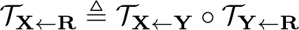
参照画像 $\mathbf{R}$ から与えられた画像 $\mathbf{X}$ への変換: $\mathcal{T}_{\mathbf{X} \leftarrow \mathbf{R}}$ を得る方法について
変換 $\mathcal{T}_{\mathbf{X} \leftarrow \mathbf{R}}$ が与えられた時、K個のkeypoint: $p_1, \ldots, p_K$ それぞれについて一次のテイラー展開を考えることができる。
ここで、$p_\cdot$ は参照画像 $\mathbf{R}$ の中のkeypointの座標を表す (ここで、$\mathbf{X}, \mathbf{S}, \mathbf{D}$ 内の座標は $z$ と表すこととする)。
以下の定式化では $\mathcal{T}_{\mathbf{X} \leftarrow \mathbf{R}}$ はそれぞれのkeypoint $p_k$ 値とその Jacobian で表すことができる。
さらに、$\mathcal{T}_{\mathbf{R} \leftarrow \mathbf{X}}$ ($\mathbf{X}$ から $\mathbf{R}$ への変換の逆変換) を求めるために、
$\mathcal{T}_{\mathbf{X} \leftarrow \mathbf{R}}$がkeypointの近傍に対し局所的に全単射であることを仮定している。
$\mathbf{D}$ のなかのkeypoint $z_k$ の近くの変換 $\mathcal{T}_{\mathbf{S} \leftarrow \mathbf{D}}$ を予測するために
まず、$z_k$ の近くの変換 $\mathcal{T}_{\mathbf{R} \leftarrow \mathbf{D}}$ を予測する。
ここで、$p_k = \mathcal{T}_{\mathbf{S} \leftarrow \mathbf{D}}$ が成立する。
このように考えると、最終的に $\mathcal{T}_{\mathbf{S} \leftarrow \mathbf{D}}$ は次のように得られる。
これは、テイラー展開を使うことで次のように変形できる
ここで、Jacobian $J_k$ は次のように表される
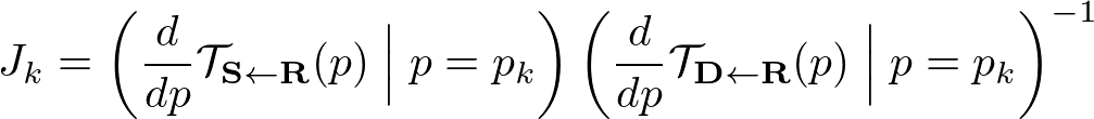
source, driving imageに対してkeypoint predictorは4つchannelを多く出力する。 これらの特徴用を用いて、対応するkeypointのconfidence mapを重みとした重み付き平均を計算することによって上の式 ($J_k$) の中の
$\frac{d}{dp} \mathcal{T}_{\mathbf{S} \leftarrow \mathbf{R}} (p) \Bigm|p=p_k$
$\frac{d}{dp} \mathcal{T}_{\mathbf{D} \leftarrow \mathbf{R}} (p) \Bigm|p=p_k$
の2つの行列の相関を得ることができる。
Combining Local Motions
それぞれのkeypointについて変換をおこなうことで、 K個のkeypointの近傍についてアラインされた、変換後の画像 $\mathbf{S}^1, \ldots, \mathbf{S}^K$を得ることができる。
また、$\mathbf{S}^0 = \mathbf{S}$ を背景として考慮する。
それぞれのkeypoointに対して、heatmap $\mathbf{H}_k$ を計算することができる。これはどの部分でそれぞれの変換が生じているかを表す特徴量である。
heatmap $\mathbf{H}_k(z)$ は $\mathbf{R} \rightarrow \mathbf{D}, \mathbf{R} \rightarrow \mathbf{S}$ のふたつの変換をもとに求められたふたつのheatmapの差として考えられる。

heatmapとK+1個の変換後 source imagewpconcatし、U-Netに入力する。 K個の部分で物体が構成され、それぞれの部分が変換されて動くというように考え、 K+1個のmaskを予測する。それぞれは 最終的なdense motionは次のように導出される
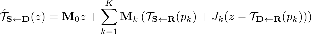
ここで、$M_0z$ は「背景」のような動かない部分として解釈できる。
Occlusion-aware Image Generation#
特徴 量マップ $\xi\in \mathbb{R}^{H' \times W'}$ 得て、これを $\hat{\mathcal{T}}_{\mathbf{S} \leftarrow \mathbf{D}}$ をもとにwarpさせる。
ここで、occlusion mask $\hat{O}_{\mathbf{S} \leftarrow \mathbf{D}} \in [0, 1]^{H' \times W'}$ でinpaintするべき場所を表す。 つまり、“occluded” された部分に対応した特徴量の影響を削減する効果をもつ。 こうして変換された特徴量マップ $\xi'$ は次のようにあらわされる
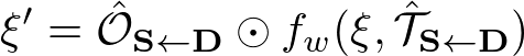
ここで、$f_w (\cdot, \cdot)$ はback-warpingを表し、$\odot$ はアダマール積を表す。 このocclusion maskは次の層に入力され、画像生成に使われる。
Training Loss#
reconstruction loss
Perceptual Lossをベースにしたロスで事前学習済みのVGG-19ネットワークを用いる。 $$ L_{rec}(\hat{\mathbf{D}}, \mathbf{D}) = \sum_{i=1}^I \left|N_i (\hat{\mathbf{D}}) - N_i (\mathbf{D}) \right| $$ ここで、$N_i(\cdot)$ はVGG-19の特定の層の i-th channel を表す。また、$I$ はその層のchannel数を表している。 これは、$\mathbf{D}, \hat{\mathbf{D}}$ をdown samplingさせることで複数のロスを取る。
Imposing Equivariance Constraint
Equivariance loss に Jacobian の制約を加えて拡張する。 この手法では、 $\mathbf{Y}$ から $\mathbf{X}$ への変換に対して、参照画像 $\mathbf{R}$ を仮定して $\mathbf{R}$ から $\mathbf{X}$ への変換と $\mathbf{R}$ から $\mathbf{Y}$ への変換を導出した。 このことを用いて、次のequivariance constraintが成り立つ
1次のテイラー展開を両辺に行うと、次のふたつの制約を得ることができる。

2つ目のこの制約は L1 loss で実装してしまうと、Jacobianの値を0に近づけてしまうという問題点がある。そのため、次のように式を書き換える。
予備実験によると、reconstruction lossとeqivariance lossの間の相対的な重みにそこまで敏感でない (あまり重要なパラメータではない) ため、すべての実験で同じ重みを採用している。
Dataset#
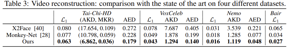
Result#
References#
- official code
