Swin Transformer: Hierarchical Vision Transformer using Shifted Windows を読む
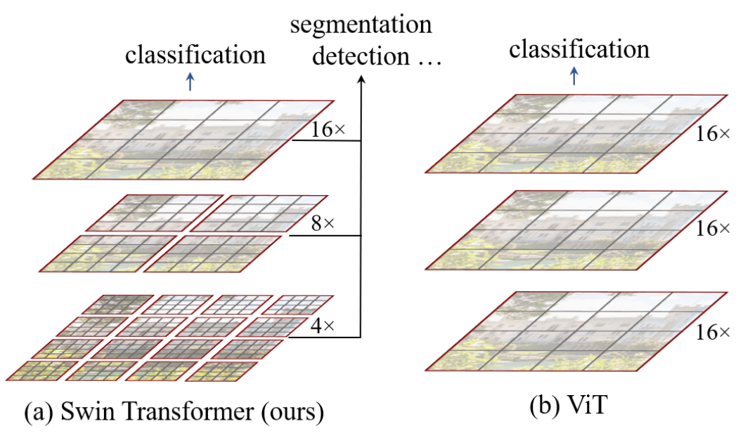
Swin Transformer: Hierarchical Vision Transformer using Shifted Windows という論文を読んでいきます (本文中の図は論文より引用) 。
Method#
Swin Transformer Block
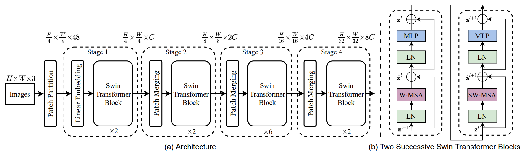
Multi-head self attention (MSA) をshifted-windowsのTransformerに置き換えることで作られる (図1 (b) 参照) 。
Shifted Window based Self-Attention#
Shifted window partitioning in successive blocks
window-basedなself-attentionはwindow間をまたいで情報を得ることができない。 そこで、shifted windowの分け方を提案する。
下図にshifted windowのやり方を表す。
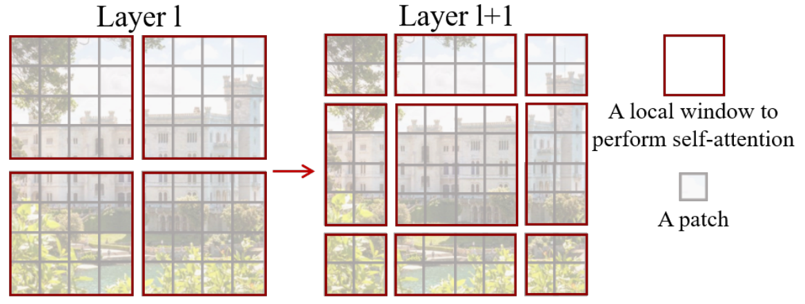
最初のモジュールは通常の分け方、つまり、左上から切り分けていく。 つまり 8×8 の特徴量を 4×4 のサイズを持つwindowに切り分ける (つまり、2×2のwindowが生成される) 。その次のモジュールではwindowが (⌊M2⌋,⌊M2⌋) だけ移動する (shifted-window)。 つまり、Swin Transformer blockでは下式のように計算される。
ˆzl=W-MSA(LN(zl−1))+zl−1,zl=MLP(LN(ˆzl))+ˆzl,ˆzl+1=SW-MSA(LN(zl))+zl,zl+1=MLP(LN(ˆzl+1))+ˆzl+1,
Efficient batch computation for shifted configuration
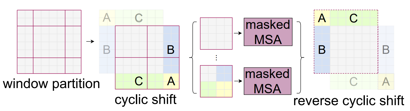
shifted windowの問題点として、windowの数が増える (⌈hM⌉×⌈wM⌉ → (⌈hM⌉+1)×(⌈wM⌉+1)) ことと、 いくつかのwindowのサイズが M×M よりも小さくなってしまうことが挙げられる。
これをナイーブな方法 (padding) ではなく解決するために、cyclic-shiftingを用いる (図3)。 このshiftを行ったあと、windowには隣接していない部分が含まれることになるが、maskingをすることでself-attentionに制限をかける。 この手法により、普通に分割したときと同じ数・サイズのwindowが生成できる。
Relative position bias
self-attentionを計算するとき、相対的なposition bias B∈RM2×M2を加える。 ここで、M2 はwindowに含まれるpatchの数を表す。
つまり、次式でattentionの計算を行う Attention(Q,K,V)=SoftMax(QKT/√d+B)V
相対的な位置は [−M+1,M−1] の範囲に収まるため、bias matrixを ˆB∈R(2M−1)×(2M−1) をのようにパラメータ化できる。 Bの値は ˆB から引っ張ってくる。
Architecture Variants#
サイズと計算量のことなる複数のモデルを作ることができる。 ここで、Swin-T、Swin-Sはそれぞれ ResNet-50、ResNet-101に近いサイズである。
- Swin-T: C=96, layer numbers = {2, 2, 6, 2}
- Swin-S: C=96, layer numbers = {2, 2, 18, 2}
- Swin-B: C=128, layer numbers = {2, 2, 18, 2}
- Swin-L: C=192, layer numbers = {2, 2, 18, 2}
ここで、C は最初のステージの隠れ層のチャンネルの数。
Experiment#
ImageNet-1K#
図4に、(a) 通常の方法で ImageNet-1Kで学習を行ったときと (b) ImageNet-22Kを使って事前学習を行ったときの結果を示す。
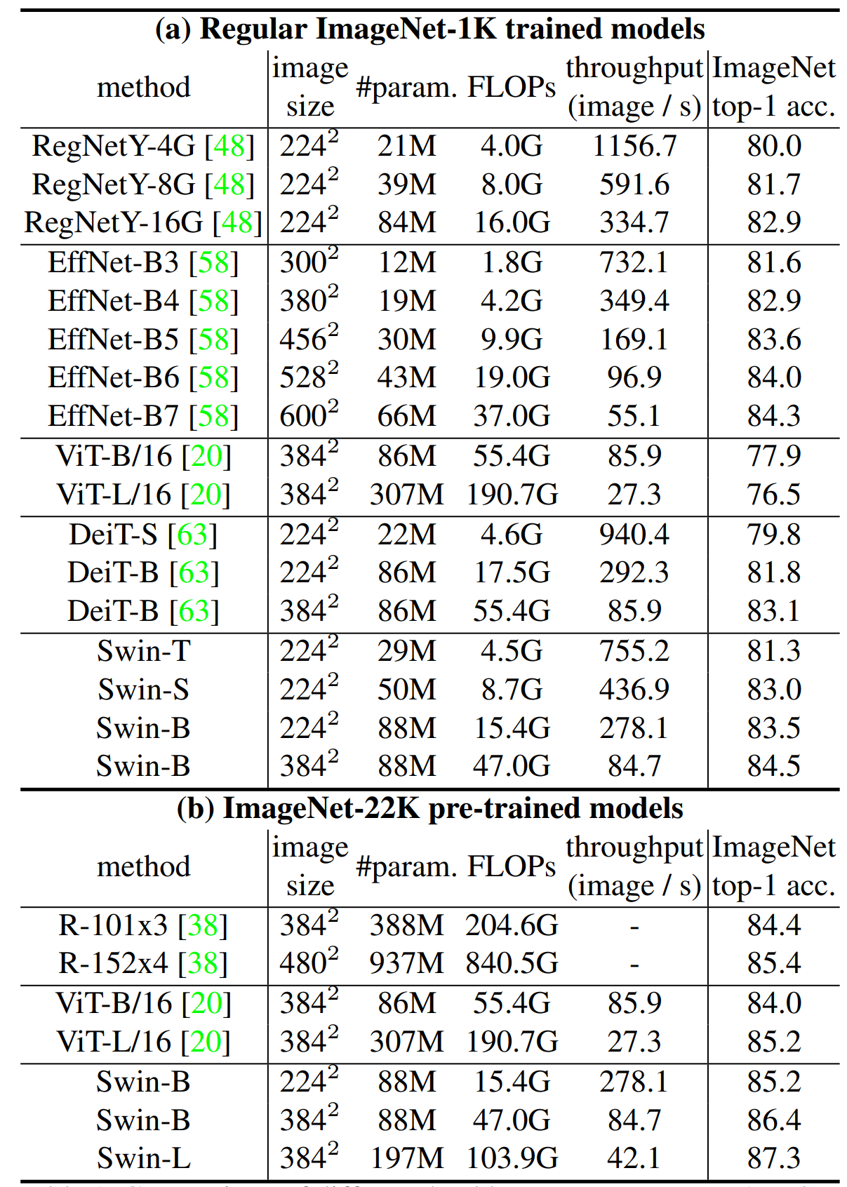
(a) について、SOTA手法である ConvNets (RegNet) や EfficientNet と比べて Swin Transformerは速度と精度のよいトレードオフ (小さくはあるが) を達成していると言える。 (b) について、事前学習を行ったとき比較手法と比べ、提案手法はとても良いトレードオフを達成している。 他にも、COCO (Object Detection) や ADE (Semantic Segmentation) についても実験を行っている (SOTAなパフォーマンスを出している)。また、それぞれのモジュールについてablation studyが行われている。
References#
Swin Transformer implementation
