Video Swin Transformer を読む
Video Swin Transformer という論文を読んでいきます (本文中の図は論文より引用) 。ざっくり言うと、Swin Transformerをそのままvideoの入力に拡張した論文です。
Method#
図1に全体のアーキテクチャを示す (Swin-Tという提案モデルの中でも小さなvariantの図) 。
全体の処理の流れはSwin Transformerとほぼ同じになるように設計されている。
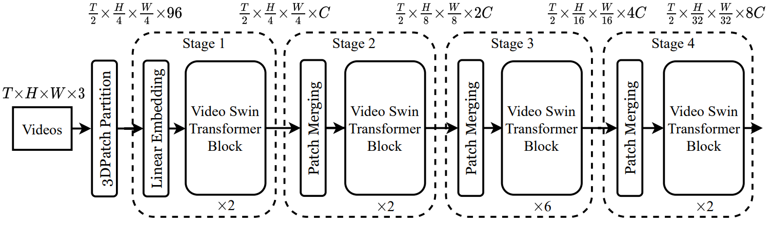
input videoは $T \text{ (frame)} \times H \times W \times 3$ のサイズを持つとする。 Video Swin Transformerでは、$2\times 4 \times 4 \times 3 = 96$次元の3D patch をひとつのtokenとして扱う。つまり、全部で $\frac{T}{2} \times \frac{H}{4} \times \frac{W}{4}$ のtokenを持つ。 その後、線形層を用いて任意の次元 ($C$とする) に拡張することができる。
各stageにおいて、時間方向にはdown-sampleを行わず、空間方向にdown-sampleを行う。また、各tokenの持つ特徴量は2倍に増加していく。
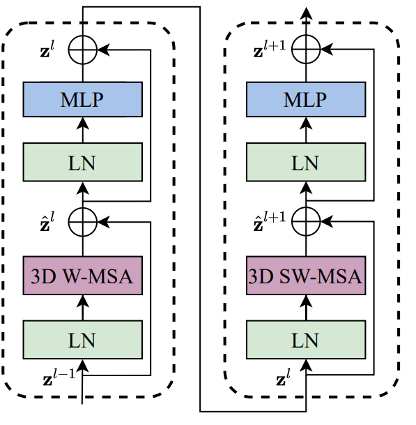
アーキテクチャの核を成すのがVideo Swin Transformer Blockである (図1) 。 標準のTransformerのmultihead self-attention (MSA) の部分を3D shifted windowに基づいたMSAに置き換えることで作られる。図の"3D W-MSA"は通常のwindowのMSA、“3D SW-MSA"はshifted windowのMSAを表す。
3D Shifted Window based MSA Module#
画像の場合と比べて、動画は時間軸を考えないといけないため、動画を扱うときには入力tokenがとても多くなる。 そのため、global self-attentionは計算量やメモリのコスト的に適していない。そこで、Swin Transformerのself-attentionモジュールにlocality inductive biasを導入したモデルを考える。
Multi-head self-attention on non-overlapping 3D windows
画像認識に用いられるようなMSAをvideoに対応するように拡張する。 $T' \times W' \times W'$ の3D tokenからなるvideoと $P\times M \times M$ の3D windowがあるとき、 つまり、input tokenは $\lceil \frac{T'}{P} \rceil \times \lceil \frac{H'}{M} \rceil \times \lceil \frac{W}{M} \rceil$ 個の重複しない3D windowに分割される。
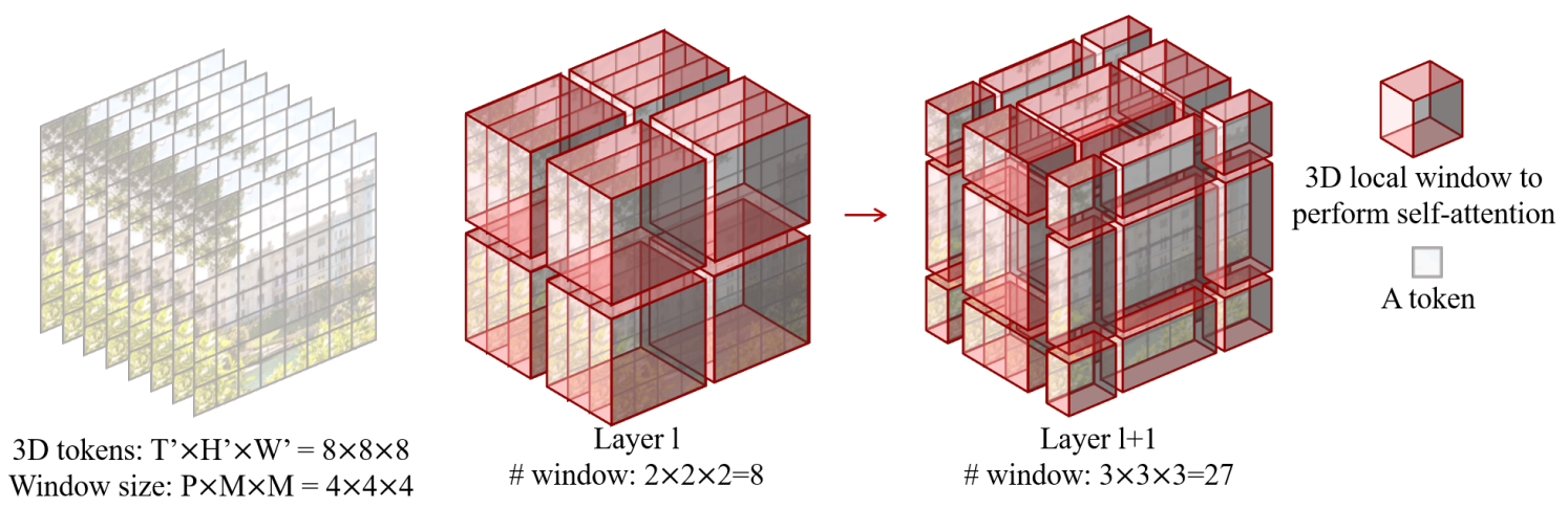
例を図2に示す。input sizeが $8 \times 8 \times 8$ で、window sizeが $4 \times 4\times 4$ のとき、層 $l$ では通常の分割法、層 $l+1$ ではwindowが $(\frac{P}{2}, \frac{M}{2}, \frac{M}{2}) = (2, 2, 2)$ tokenだけシフトする。このようにするとwindowの数が増えてしまう ($3 \times 3 \times 3 = 27$ になる) が、Swin Transformerと同様に処理することで8個のままになる。
このshifted windowを用いてVideo Swin Transformer blockでは次のように計算が行われる (Swin Transformerと同様)
\begin{align*}
\hat{\mathbf{z}}^l &= \text{3DW-MSA} (\mathrm{LN}(\mathbf{z}^{l-1})) + \mathbf{z}^{PyTurboJPEGl-1}, \\
\mathbf{z}^l &= \mathrm{FFN} (\mathrm{LN}(\hat{\mathbf{z}}^{l})) + \hat{\mathbf{z}}^{l}, \\
\hat{\mathbf{z}}^{l+1} &= \text{3DSW-MSA} (\mathrm{LN}(\mathbf{z}^{l})) + \mathbf{z}^{l}, \\
\mathbf{z}^{l+1} &= \mathrm{FFN} (\mathrm{LN}(\hat{\mathbf{z}}^{l+1})) + \hat{\mathbf{z}}^{l+1},
\end{align*}
3D Relative Position Bias
3Dの相対的なbias $B \in \mathbb{R}^{P^2 \times M^2 \times M^2}$ をAttentionの計算時に加える。 \begin{align*} \text{Attention}(Q, K, V) = \text{SoftMax}(QK^\mathsf{T} / \sqrt{d} + B) V \end{align*}
相対的な位置は時間方向に $[P + 1, P - 1]$、高さ・幅方向に $[-M + 1, M - 1]$ の中に収まることを利用し、biasを $\hat{B} \in \mathbb{R}^{(2P-1) \times (2M - 1) \times (2M-1)}$ のようにパラメータ化できる。
Architecture Variants#
サイズと計算量のことなる複数のモデルを作ることができる。
- Swin-T: $C=96$, layer numbers = {2, 2, 6, 2}
- Swin-S: $C=96$, layer numbers = {2, 2, 18, 2}
- Swin-B: $C=128$, layer numbers = {2, 2, 18, 2}
- Swin-L: $C=192$, layer numbers = {2, 2, 18, 2}
Result#
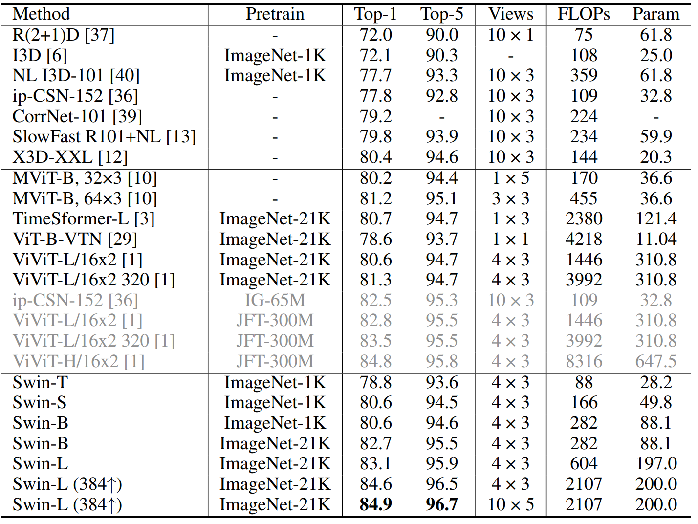
Kinetics-400に対して実験を行った結果、ImageNet-1Kで事前学習を行ったSwin-Sが MViT-B比べて計算量は同様であるものの、良い結果 (小さくはあるが) を残している。また、ConvNet X3D-XXLと比べるとかなり良い結果を残している。ほかのモデル (variants) も計算量を削減しつつ比較手法に対して良い結果を出している。
他に、Kinetics-600とSomething-Something v2での実験、ablation studyが行われている。
References#
Video Swin Transformer implementation
